It goes without saying that PostgreSQL, MondoDB, Redis, and all other database management systems require efficient methods for managing and querying their stored databases. A similarity between nearly all of these database management systems is that they make use of one of the most flexible and powerful data structures: the segment tree.
A Segment Tree Example
To demonstrate the effectiveness of the segment tree, let’s use it in an example, that acts as a continuation from last week’s post about sparse tables. After John Code (our hiker from last week) maps out a mountain range and all of the various peaks, he ends up with a new set of data indicating the number of people that visited each landmark over the past week:
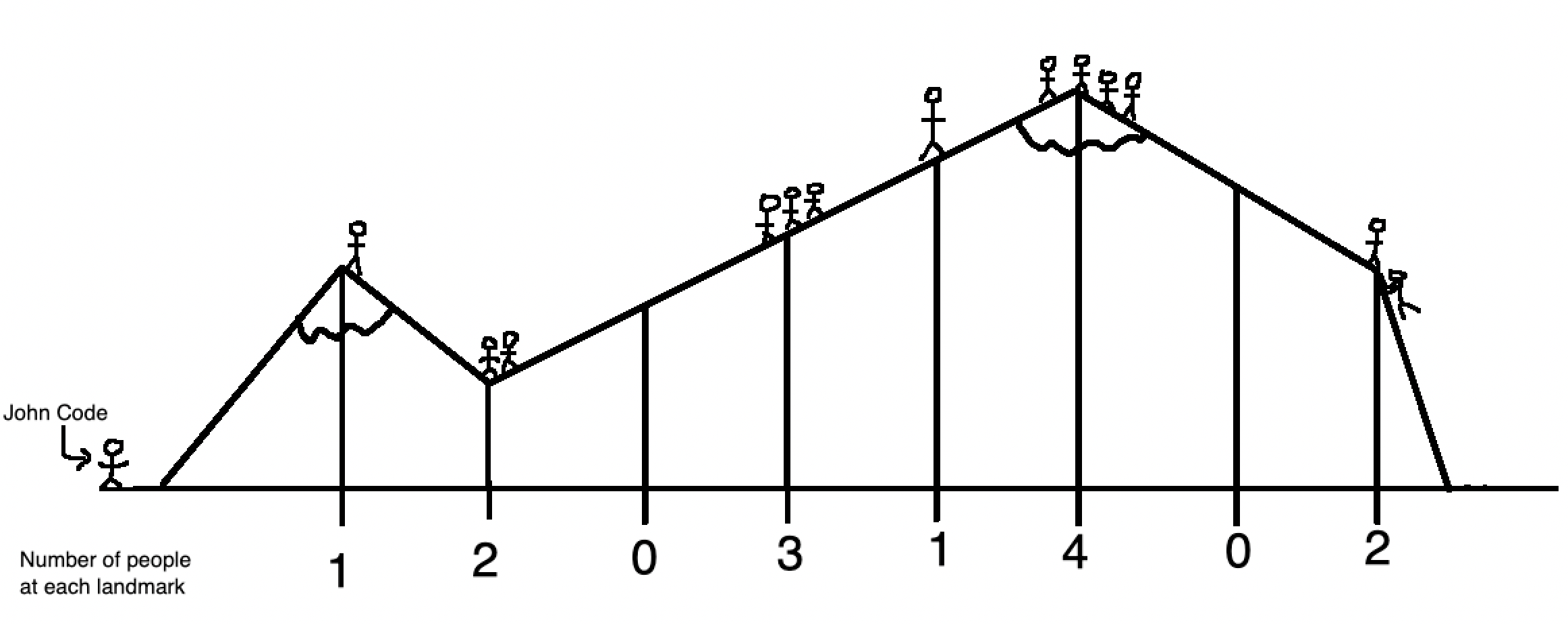
These are the measurements expressed in an array:
| Index # | 1 | 2 | 3 | 4 | 5 | 6 | 7 | 8 |
|---|---|---|---|---|---|---|---|---|
| Number of tourists | 1 | 2 | 0 | 3 | 1 | 4 | 0 | 2 |
Now John is interested in which parts of the mountain range are the most popular. To do this, he queries the sum of various subarrays. For example, the subarray representing the part of the mountain range from landmark 3 to 5 saw \(0 + 3 + 1 = 4\) people visit last week, whereas the subarray representing the part of the mountain range from landmark 1 to 4 saw \(1 + 2 + 0 + 3 = 6\) people visit last week. He then records all of these measurements in a database, and now let’s see how such queries can be computed efficiently.
To create the segment tree, we are going to compute the sums for only some of the subarrays. First, we create a node for every single measurement made, representing the trivial sum values for every subarray of length 1:

Now we compute the sum values for the subarrays of length 2 by summing every pair of consecutive nodes like below:
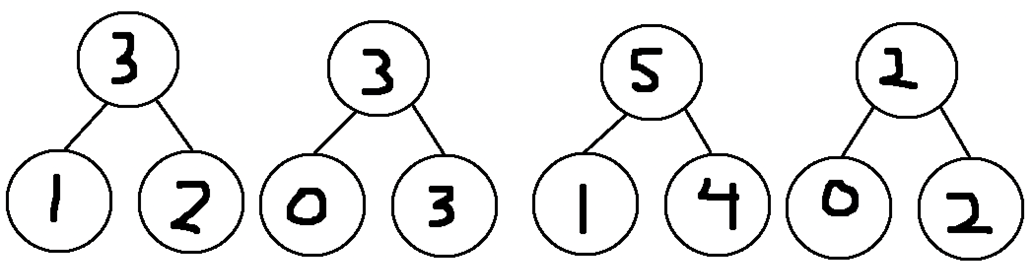
This new row now contains the sums for the subarrays with indexes going 1 to 2, 3 to 4, 5 to 6, and 7 to 8. Repeat this step with the new nodes created to get the sum values for subarrays of length 4:
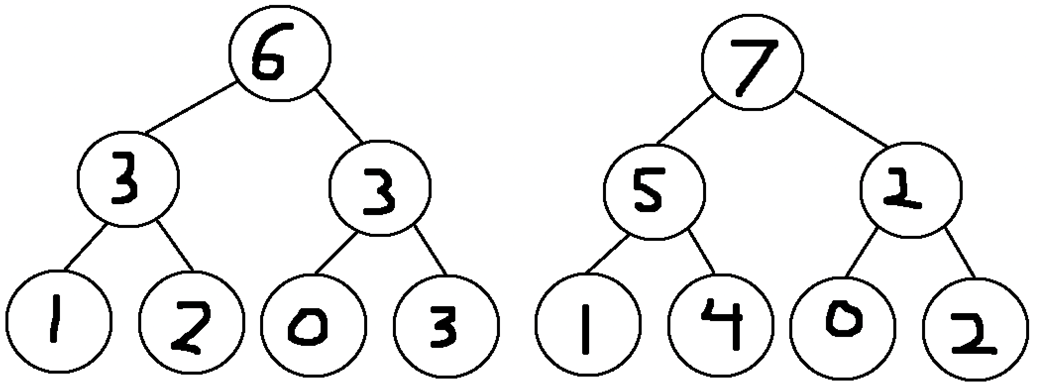
And now finally with the two nodes for the subarrays with indexes going 1 to 4 and 5 to 8, create the top layer of the segment tree representing the sum value for subarrays of length 8 (ie. the entire array):
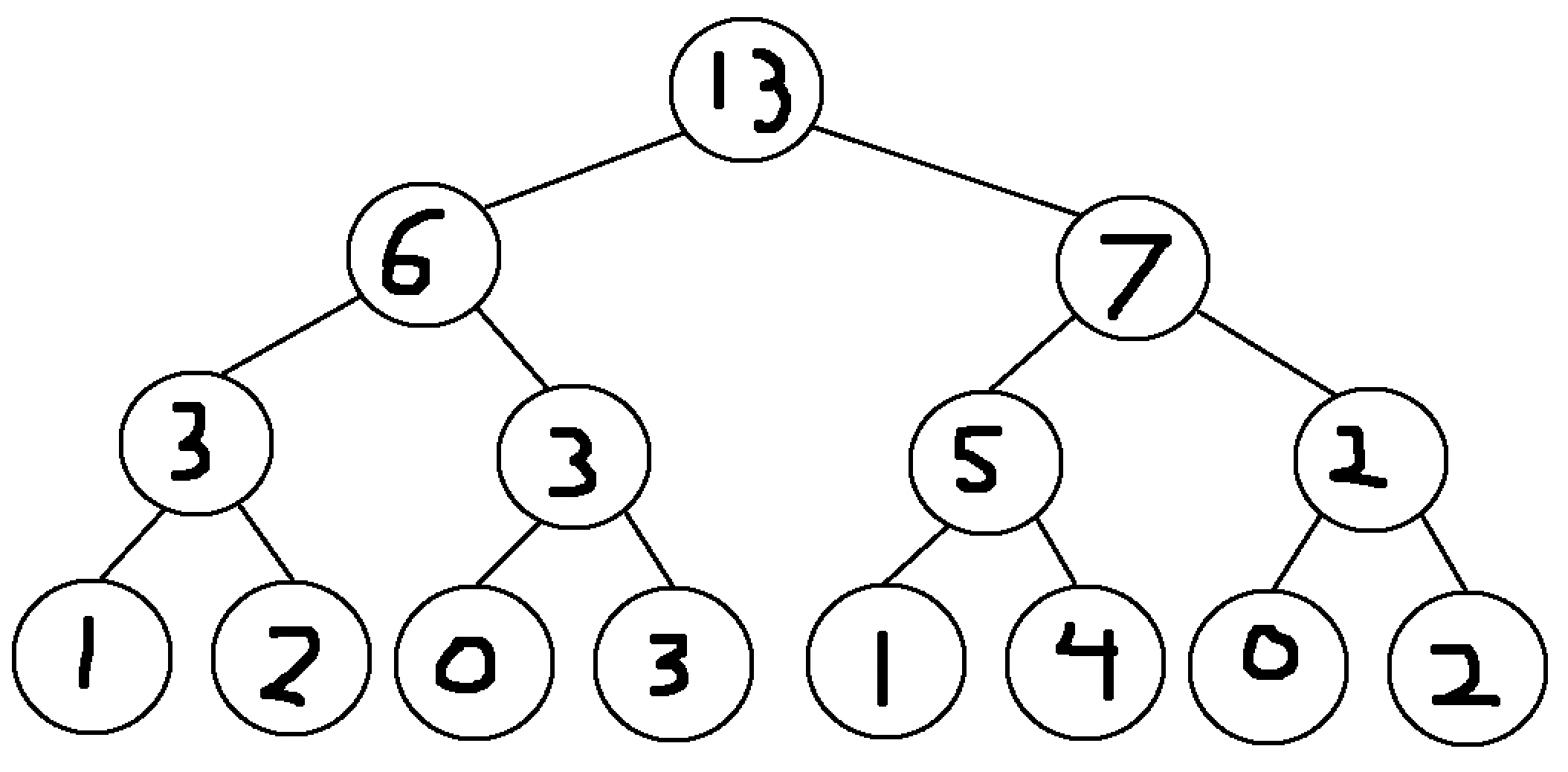
This segment tree can now be used to compute the sum of any subarray by choosing nodes greedily, meaning that the nodes that cover the largest subarrays are chosen first to minimize the number of nodes involved. For instance, if the sum of the subarray from index 1 to 7 was to be computed:
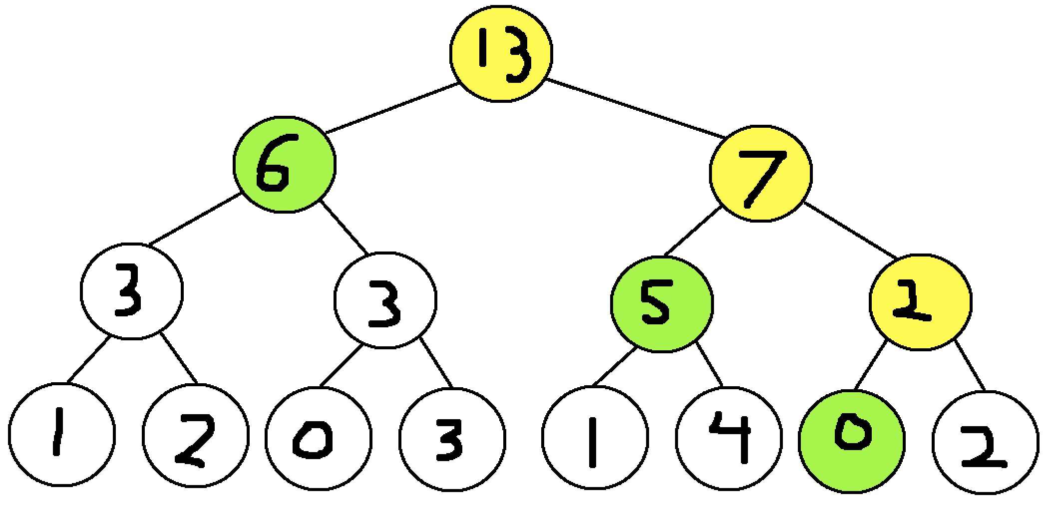
The yellow nodes indicate nodes that are only partially included in the subarray range. These nodes are not included in the sum but are instead searched deeper to their child nodes. The green nodes indicate nodes that are fully covered by the subarray range, so for maximum efficiency, these nodes are added to the sum and no further searching is required. For this example, the sum of the subarray from index 1 to 7 is \(6 + 5 + 0 = 11\).
With efficient node selection, at most one node from each layer is going to be selected. This means in a much larger case, if John Code’s robot made a million measurements in total, then because the number of nodes in each layer is divided by two each time, such a segment tree would have only 21 such layers, meaning that ANY subarray sum for an array of one million values can be computed by just adding at most 21 values together! A segment tree of that size would consist of \(1000000 + 500000 + 250000 + ... + 2 + 1 \approx 2000000\) nodes, so while there is a substantial precomputation cost, if multiple subarray sums are required, this is a much faster method than burte forcing every query. Generally, for an array of \(n\) elements, a segment tree will create roughly \(2n\) nodes, and will require summing up at most \(\text{log}_2(n)\) nodes to compute a subarray sum. In big-O notation, this means the amount of time to create a segment tree scales linearly with the size of the array and can be represented as \(O(n)\), while the time needed to complete a single query scales logarithmically with the size of the array and can be represented as \(O(\log n)\).
Database Usability of Segment Trees
Technically, there are simpler methods to finding the sum of any subarray that are equally as fast or even faster, such as prefix sums. However, suppose that John later finds there was an error in his data, and that landmark 5 actually had a lot more people there last week, updating the array to something like below:
| Index # | 1 | 2 | 3 | 4 | 5 | 6 | 7 | 8 |
|---|---|---|---|---|---|---|---|---|
| Number of tourists | 1 | 2 | 0 | 3 | 100 | 4 | 0 | 2 |
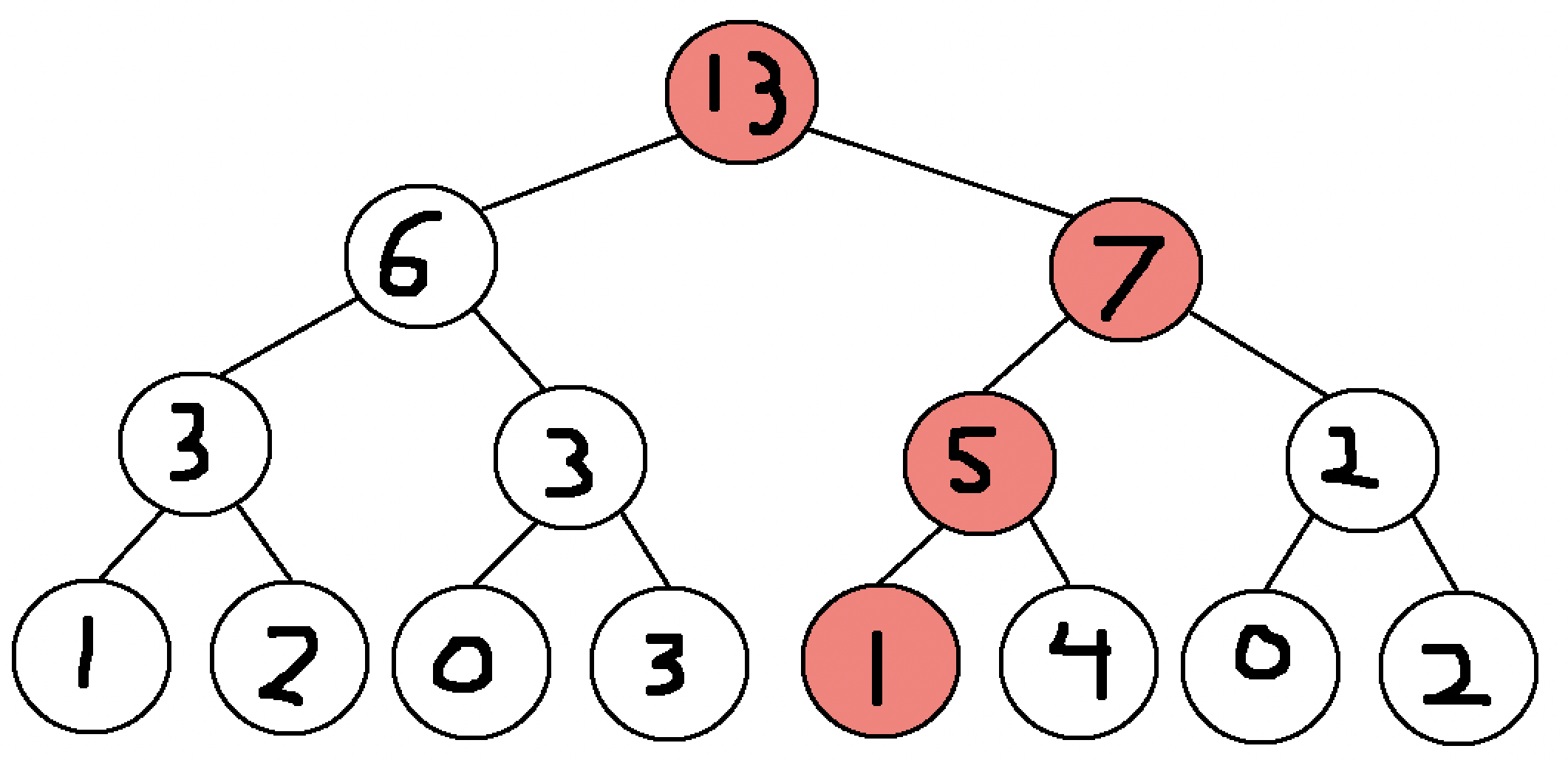
These data updates can be common in a database context, and what makes segment trees useful is how they handle these changes. First, we highlight all nodes that are affected by this change in the previous segment tree red. These nodes include the base node tracking the sum of the subarray from index 5 to 5 in the bottom layer, and each subsequent parent node up to the top.
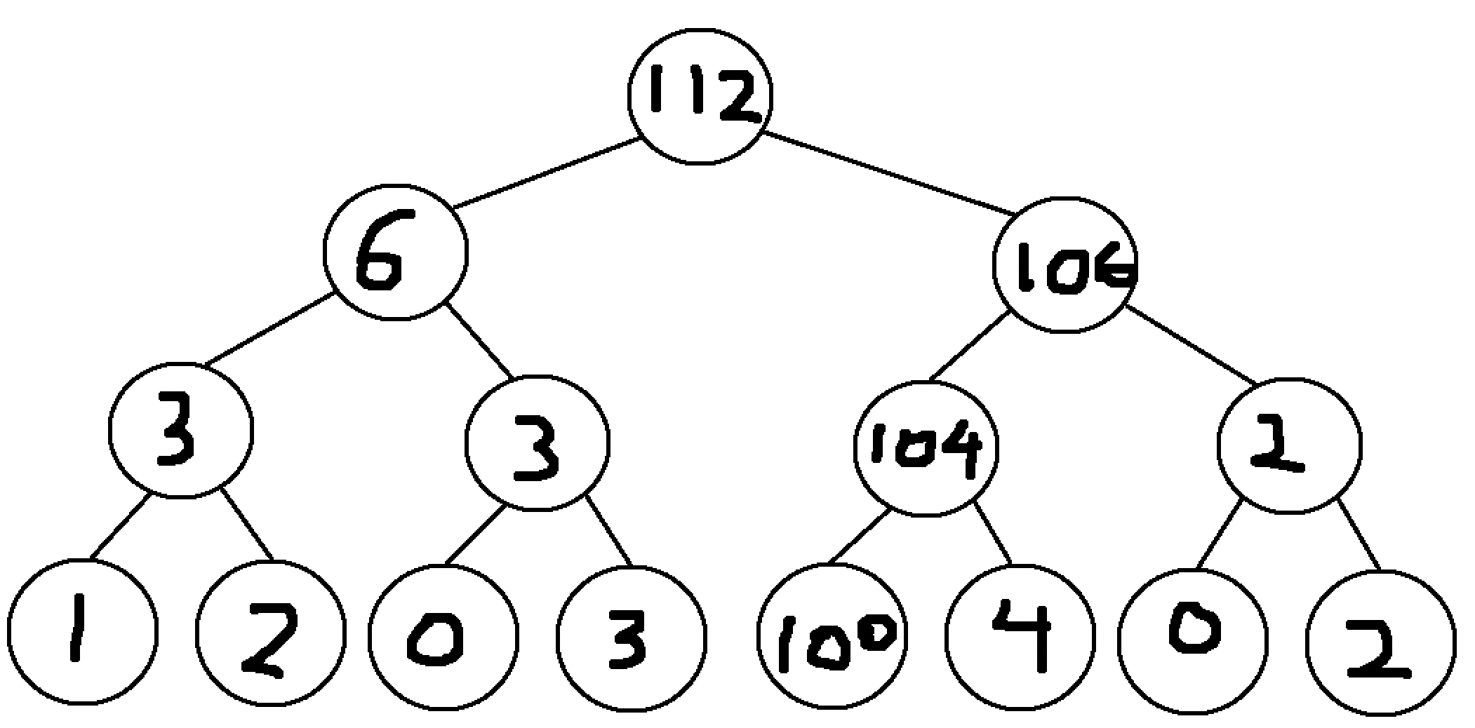
Now starting from the bottom node in this tree, update each node: - The sum of the subarray from index 5 to 5 is now 100 (previously 1) - The sum of the subarray from index 5 to 6 is now 104 (100 + 4) - The sum of the subarray from index 5 to 8 is now 106 (104 + 2) - The sum of the subarray from index 1 to 8 is now 112 (6 + 106)
Now with this updated segment tree, the subarray sum queries can be computed in the same way as before. Even with a much larger tree, the number of nodes that need to be updated will always be equal to the number of layers in the tree, thus meaning that the amount of time needed to perform such an update scales logarithmically with the array size. This means that this is roughly as fast as the \(O(\log n)\) operation used for finding a subarray sum.
Conclusion
In short, segment trees are a data structure based solution that explains how database management systems are capable of processing database queries in an efficient manner. The subarray sum problem is just one of the many applicable uses of segment trees, and further explanation as well as a code implementation of the structure can be found on cp-algorithms, which is one of the largest information bases for various data structure and algorithmic concepts used in competitive programming.